A RELATIONAL GEOMETRIC MODEL FOR VARIATIONAL GEOMETRY
(Arbeitsbericht)
Chun Du, Roland Berling, Manfred Rosendahl
University of Koblenz-Landau,
FB Informatik,
Rheinau 3-4, 5400 Koblenz,
F. R. Germany
ABSTRACT:
This paper presents a relational geometric model for variational geometry. A geometric object in a relational geometric model is represented based on its geometric relationship to other geometric objects and is unilaterally dependent on these objects. Through the unilateral dependency among the geometric objects local dimensional changes can be propagated to the whole model easily so that the consistency of the geometric model is maintained. A new concept called late constraint is introduced to deal with the situation of cyclic dependency among the geometric objects. By using late constraints the number of constraint equations which have to be solved simultaneously can be reduced to a minimum by the user.
KEYWORDs:
Geometric model, geometric constraint, geometric relationship, dimension, variational geometry, geometric object, Geometric Modelling Primitive(GMP), late constraint.
1. INTRODUCTION
Automated variation of design models is an important function of CAD systems nowadays. Many approaches have been presented which meet this requirement by dealing with the variation of the geometric model[1,3,5,6,7,8,9,11,12,13]. In these approaches metric relationships between pairs of geometric objects (also called dimensions) are treated as geometric constraints. By manipulating the geometric constraints the following tasks can be performed:
1) to generate a geometric model automatically when sufficient geometric constraints and information about topological descriptions of and geometric relationships among geometric objects are given;
2) to maintain the consistency of the geometric model, when one or more dimensions of the model have changed.
Obviously, not only metric but also geometric relationships among geometric objects have to be considered as indispensable parts of the geometric model if the variations of the geometries are dealt with. We call them geometric constraints of the geometric models.
There are two popular methods of approaching variational geometry. One is to translate each constraint into an equation and then to solve a system of equations derived from a model simultaneously. The unknowns in the equations are coordinates of the characteristic points of the model[6,7,12]. Another way is to use geometric reasoning mechanism in which the dimensions and geometric relationships are defined as either facts or rules and represented in the form of Prolog-clauses[1,2,3,13]. These facts or rules are used to do the inferences on the symbolic level to maintain the consistency of the model. These two methods have a common character: geometric constraints are defined and exist separated from the geometric model and are used to control the behaviour of the model.
In this paper another method in the variational geometry is presented. The character of this method is to embed the geometric constraints and their maintenance processes in the geometric models. In most cases, a geometric model constructed with this method can remain consistent by itself through holding the validities of the geometric constraints when some of the dimensions have changed. This is realised by defining each geometric object as a product of its relationships to other geometric objects. Any changes in the related objects of an object causes also a change in this object through the relationships among them so that the relationships stay invariable.
Section 2 discusses the relationships among the geometric objects and how the geometric objects are represented; section 3 discusses the issues of geometric modelling; in section 4 the maintenance of the consistency of the geometric model are discussed; section 5 is a case study to show how to construct geometric models with our method; section 6 introduces the implementation of a CAD system.
2. THE GEOMETRIC OBJECTS
2.1 What is a geometric object
Following objects are defined as geometric objects:
- Value (dimension), e.g. coordinate, length, distance, radius or angle.
- Point,
- Line,
- Circle, and
- Arc.
In the following discussion we shorten geometric object to object.
2.2 The relationships among geometric objects
There are various kinds of geometric relationships among geometric objects. The following geometric relationships are dealt with in our approach:
1) Structural relationship
This is a 'composed-of' relationship between geometric objects according to the normal concept of geometry, i.e. an object is a component of another object. For example, the centre point and radius are components of the circle.
2) Dimensional relationship
This is a numerical relationship among the dimensions. For example, the radius of a circle is the distance between the two existing points or the length of an existing line.
3) Positional relationship
This is a spatial relationship among the objects in 2-dimensional space. There are some standard positional relationships: tangency, parallelism, perpendicularity, symmetry, relative location and intersection.
These three kinds of geometric relationships cause the logical dependencies among the geometric objects. Structural relationship always causes unilateral dependency, i.e. an object is dependent on the other objects involved in the structural relationships. For example, a circle is dependent on two other objects: centre point and radius. Dimensional relationship also brings about, besides unilateral dependency, bilateral dependency among the objects, i.e. two objects involved in a dimensional relationship influence each other. For example, if the radius of a circle is equal to the length of a line, they depend on each other. Positional relationship causes mainly bilateral dependency among objects. But sometimes it also brings about unilateral dependency. For example, an intersection point is dependent on the objects which intersect at this point.
2.3 Modelling the geometric objects and geometric relationships
How to model all kinds of geometric objects and geometric relationships is the basic issue of variational geometry. The crucial point is how to record and represent the geometric relationships. Conventional approaches represent geometric objects and geometric relationships separately. Geometric relationships are represented as equations or rules outside the geometric model which are then used to control the behaviour of the model.
Our approach tries another way. We represent geometric objects and relationships in an integrated form. A geometric relationship among a group of geometric objects is represented as unilateral dependency of a certain object in the group on the other objects of the group. Strictly speaking, we represent a geometric relationship through the fact that the geometric data of a certain object involved in this relationship is evaluated on the basis of the data of other objects involved in the same geometric relationship and the property of this relationship. In other words, we represent a geometric relationship as an evaluating operation.
Structural relationship can be directly represented with this method because one object involved in a structural relationship is definitely unilaterally dependent on other objects. For example, the structural relationship between a circle, its centre and radius can be represented by the fact that the data of centre point and radius are the geometric data of this circle. Dimensional and positional relationship cannot be represented directly with this method because they mainly cause bilateral dependencies between the objects. In order to achieve a common form for all types of relationships, we represent them indirectly with an operation which causes the specified relationship during the evaluation. This operation states a kind of unilateral dependency between its arguments and the resulted object, as in structural relationship. For example, a dimension relationship "dimension R1 is two times as long as the dimension R2" can be represented by an evaluating operation which contains an calculation R1:=2 * R2; a positional relationship "a line is tangent to two circles" can be represented by an evaluating operation which contains the process to compute the end points of the line which are also the tangent points using the data of the two circles.
As a result of the discussion above, a geometric object can be represented by an evaluating operation which evaluates its geometric data on the basis of a group of other geometric objects. Each object therefore is dependent on some other objects. It can be represented either
1) by its components, e.g. a circle is represented by its centre and its radius; or
2) as a mathematical expression, e.g. a dimension R1 can be represented as an expression (2 * R2) if R1 is required to be double as long as the dimension R2; or
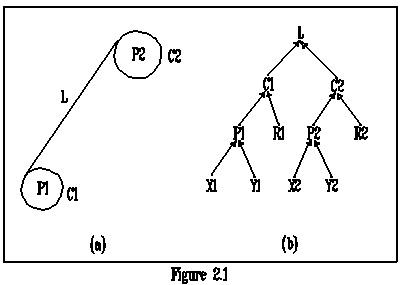
3) as an object whose geometric data is obtained by solving a set of equations describing how it is positional related to other objects, e.g. a line can be represented by two circles if this line is tangent to these circles. see figure 2.1(a).

The two tangent points, which determine the position of the line, can be calculated by running a predefined evaluating process which find a solution for this situation. Figure 2.1(b) shows the dependency relationships among the participated geometric objects. The arrow-line shows the direction of dependency.
There are also geometric objects which do not depend on any other geometric objects. For example a dimension may be an absolute data. These objects can also be represented with our method if we assume that the evaluating operations for them are empty.
So far we have set up an unified method to represent geometric objects and geometric relationships. The advantage of this method is that the relationships are embedded in the objects. Because the representation of geometric objects need geometric relationships and vice versa we have found an integrated way to model the geometric objects and the geometric relationships. Now we introduce how the objects are modelled in a CAD system.
2.4 THE DEFINITION OF GEOMETRIC OBJECTS
We differentiate at first the types (or classes) of the objects from the objects which appear in the geometric models. We say that a geometric object in a geometric model is an instance of its type (or class). We call the types (or classes) Geometric Modelling Primitives (GMPs) and discuss the definitions of the geometric objects and relationships on the GMP level.
Five absolute GMPs are defined. They are value, point, line, circle, and arc. Value is a numerical data; point is a 2-tuple of numerical data representing a position in the 2D space; line is defined by two 2-tuples of numerical data representing the two ends; circle is defined by a numerical data representing the radius and a 2-tuple of numerical data representing the centre; arc is defined by three numerical data representing the radius, the start- and end- angle, and a 2-tuple of numerical data representing the centre. The structure of each absolute GMP is called geometric character of this GMP.
A group of conditioned GMPs are also defined. Each conditioned GMP not only has the same geometric character with respect to one of the absolute GMPs, but also the information about how it is constructed. This information includes:
(a) a computing process which computes the data of this GMP,
(b) one or more GMPs named support GMPs on which this GMP is dependent.
The computing process of (a) corresponds to the evaluating operation in section 2.3. It uses the support GMPs in (b) and the geometric relationship to compute the data of this GMP. For example, a conditioned GMP line_2o may contain following information:
(a) procedure to compute the coordinates of two ends,
(b) two support GMPs, for example two circles.
The procedure of (a) knows how to compute the coordinates so that this GMP line_2o will be tangent to the support GMPs if they are circles.
Figure 2.1(a,b) shows how the conditioned GMP line_2o is defined. Figure 2.2 shows the definitions of the conditioned GMPs pointRef and pointPolar.

Because a certain kind of geometric object can have many kinds of geometric relationships with other kinds of geometric objects, there have to be many different representations for a certain geometric object, e.g. the points in figure 2.2. Therefore there are a number of GMPs who have the same geometric character but different kinds of support GMPs and geometric relationships with the support GMPs. We say that this group of GMPs belong to a GMP-class. There are five GMP-classes so far, based on the five absolute GMPs. Each conditioned GMP of a GMP-class is derived from the absolute GMP of this GMP-class which means that this conditioned GMP inherits the geometric character from the absolute GMP of this GMP-class. For example, The points defined in figure 2.2 belong to the GMP-class point and is derived from the absolute GMP point.
Up until now we have only discussed the definitions of the conditioned GMPs. The dependency of conditioned GMPs on their support GMPs is confined to acyclic dependency. There is also a kind of GMP which deals with cyclic dependency. It is used to set extra dimensional restrictions on conditioned objects. For example, it could be used to fix the length of the line L in figure 2.1(a). This kind of constraint is called late constraint because it is mostly assigned to the objects after they have been created. The late constraints belong to the GMP-class value. We call the conditioned object which the late-constraint is assigned to a late-constrained-object. Late-constrained-objects can only be of type value, e.g. the length of a line.
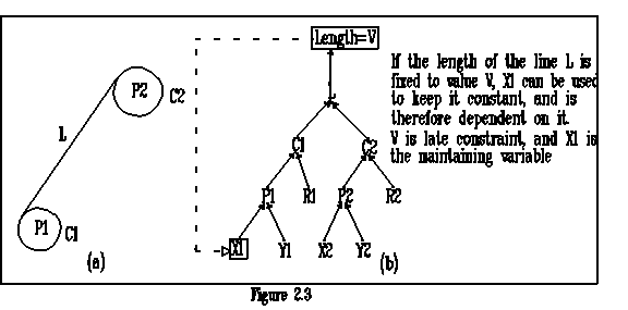
A late constraint causes cyclic dependency among the geometric objects because as an extra independent dimensional constraint it influences the original dimension of a late-constrainted-object and thereby the support objects of it which again determine the original dimension. For example, when the length of the line L in figure 2.3(a) is fixed, the positions and radii of both circles C1 and C2 are also restricted. Changing one of them leads to a irregular value for the length of the line L which does not agree with the fixed length. Figure 2.3(b) illustrates the situation of cyclic dependency. In order to maintain the consistency of the late constraint a free dimension which directly or indirectly supports the late-constrained-object should be selected as a maintaining variable. A maintaining variable of a late constraint has the following tasks:
1) When the value of the late constraint has changed the maintaining variable should also be changed so that one of the support objects of the late-constrained-object gets the new data which leads to a consistent late constraint.
2) When the support objects of the late-constrained-object have changed the maintaining variable should be changed so that the late constraint remains satisfied.
A dimension is no longer free if it is selected as the maintaining variable of a late constraint. Figure 2.3(b) shows an example where the coordinate X1 is selected to be the maintaining variable if the length of the line L is fixed to be the value V.
3. CONSTRUCTIVE GEOMETRIC MODELLING WITH GMPs
During the process of geometric modelling the GMPs are treated as types (or classes). Each geometric object in a geometric model is an instance of one of the GMPs. An absolute object is an instance of the absolute GMP; a conditioned object is an instance of the conditioned GMP. A geometric model is composed of conditioned objects, absolute points, absolute values and late constraints.
According to the definition, a geometric object is unilaterally dependent on some other geometric objects. This dependency is acyclic and leads to certain sequences in constructing a geometric model. For example, before a circle is created in a geometric model a point should have existed in the model which can then be used as the centre point of the circle. We call this kind of modelling process constructive modelling.
Dimensions are treated as geometric objects and are directly used in geometric modelling. Dimensional constraints can be properly assigned with regard to the user's intention and are totally involved in the geometric models. Under-dimensioning is therefore not possible. Over-dimensioning can only happen when late constraints are assigned.
It is necessary to use late constraints only when the model can not be constructed in sequential order because of the circular dependencies in the model. Therefore a model without circular dependencies is first constructed and the remaining properties are put into the model by means of late constraints.
4. MAINTAINING THE CONSISTENCY OF THE GEOMETRIC MODEL
To maintain the consistency of a geometric model means to preserve the invariable geometric properties e.g. the geometric relationships or fixed dimensions when some of the dimensions have changed. This is done by evaluating the geometric model in our approach (see also [4]).
Evaluating a conditioned geometric object means to calculate its data by running its computing process. Because of the unilateral dependency of conditioned objects on their support objects, the data of a conditioned object can only be calculated by using the data of its support objects. This calculation is performed by the computing process of the conditioned objects. Therefore any change in the support objects results in changing the conditioned object through its evaluation so that the geometric relationship among them stays invariant.
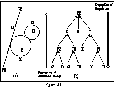
Evaluating the geometric objects can propagate the changes of dimensions in the geometric models. This is enabled through the propagation of computation of geometric objects. The propagation of computation is a recursive process of running the computing processes of the support objects in each geometric object until those objects are reached which either have no computing process, e.g. absolute objects, or which have already been computed. Through the directed propagation of computation any changes of the data of an absolute object can be propagated back to those conditioned objects which are directly or indirectly supported by it. This is the propagation of new dimensions. These two propagation processes work in opposite directions. Figure 4.1(a) shows a sample model and figure 4.1(b) shows the dependency relationships among its component objects and the directions of the two propagation processes.
The evaluation of a late-constrained-object is more complicated then the evaluation of other geometric objects because of the cyclic dependency among the late-constrained object, its late-constraint, and the maintaining variable of the late-constraint (see figure 2.3(b)). An iterative procedure is needed to find an appropriate value for the maintaining variable to satisfy the late-constraint. More then one late constraint can exist in a model at the same time and some of them may be related to each other when the maintaining variable of one late constraint is the support object of another late-constrained-object. The related late constraints should be satisfied simultaneously, which means we have to solve a set of (non-linear) constraint equations where the unknowns are the maintaining variables. For each geometric model there is one process to satisfy all late constraints (independent and related) by using Newton-Raphson iterative method. When evaluating a geometric model this process will not be run until all other objects of the model have been evaluated.
Because the late constraints are necessary only when the geometric model can not be constructed in sequential order any more and because they are assigned to the model after the main part of the model has been sequentially constructed, the number of the constraint equations which have to be solved simultaneously can be reduced by the user.
Late constraints can also be used to intentionally change the data of conditioned objects, e.g. to move the circle C2 of figure 4.1(a) to an intended new position by changing two absolute values X1 and Y1 of figure 4.1(b). In this case, the new position of the circle C2 can be seen as a temporary late constraint. The free variables X1 and Y1 are then temporary maintaining variables of it.
5. CASE STUDY
Some examples are presented in this section to show how the geometric models are constructed and how the geometric constraints are managed in our approach.
The first example is to construct a triangle whose three sides have definite lengths respectively as shown in figure 5.1(a).

One possible construction is to use auxiliary circles. In the model, P1 is defined as a free point. P2 is defined as a polar point whose origin is P1 and the distance between them is d1. The angle is free. P3 is defined as an intersection point of two auxiliary circles C1 and C2 which take the points P1 and P2 as centre point and value d3 and d2 as radius respectively. Figure 5.1(b) is a DAG illustrating how the points of the triangle are constructed.
This example demonstrates that with the help of auxiliary objects the late-constraints can be avoided with our constructive modelling method, i.e. we can construct some complicated geometric models without having to solve an equation system.
There is also another possible construction in which a late constraint is used. Figure 5.1(c) shows how the points of the triangle are constructed. In the model, P3 is defined as a free point. P1 and P2 are defined as polar points with a common origin P3. The distance between the origin P3 and the points P1 and P2 are d3 and d2 respectively. The angles w1 and w2 of P1 and P2 are free. We define also an object V1 of type 'value2p' which is the distance between P1 and P2. A late constraint d1, marked with a square in the picture, is assigned to this object which demands that the object V1 has the value d1. Any of the free values X3, Y3, w1 and w2 can be selected as maintaining variable of the late constraint d1.
The second example is to construct a structure shown in figure 5.3(a) where a box is placed in a square hole. One corner of the box touches the bottom of the hole, another corner of it touches one side of the hole and one side of it lies on the edge of the hole. All the objects are fully constrained.

First we assume that the line L1, the point P3 and the distance d1 are known. We select a point P1 on the bottom line so that the point P2 can then be defined as an intersection point of L1 and the auxiliary circle C which has the centre point P1 and the radius d1. Then we define the value w1 as the angle of the point-pair (P1,P2) and the value w2 as the angle of the point-pair (P1,P3). At last we define a value W of type 'expression' which is the difference between w1 and w2. Now we assign a late constraint '90' to the value W which means that the value W must have the data '90'. We select then the x-coordinate X1 of the point P1 as the maintaining variable of this late constraint. There is therefore one extra equation in the model. During solving this equation X1 is varied so that W reaches the value '90'. Figure 5.3(b) shows how the points and values are constructed. The object marked with a square is the late constraint and the object marked with a circle is the maintaining variable.
The model in this example cannot be completely constructed without late constraint. This example shows that
1) late constraints are necessary and can be well integrated in the constructive modelling process; and
2) the combination of constructive modelling and late constraints can reduce the number of the equations which have to be solved simultaneously.
6. OBJECT-ORIENTED IMPLEMENTATION OF A CAD SYSTEM
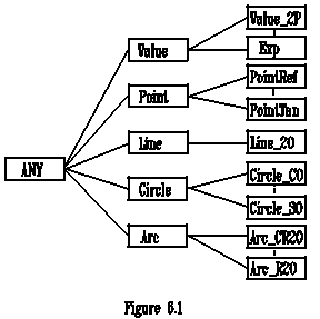
A 2D CAD system -- RelCAD (Relational CAD) has been implemented based on the concepts discussed in this paper, using object-oriented programming techniques (also see [4] and [10]). All the GMPs are implemented as classes. There is a system-wide superclass defining the common properties and operations for all other classes. The classes of conditioned objects are defined as subclasses of the classes of absolute objects. Figure 6.1 shows the class hierarchy. Due to the diagram size, only some of the classes of conditioned objects are presented.
An example of class definition, written in Turbo Pascal 5.5, is shown below:
line = object(item)
x1,y1,x2,y2:real;
constructor init(xx1,yy1,xx2,yy2:real);
procedure compute(kind:tvalkind);virtual;
.
.
end;
line_2o = object(line)
alter:integer;
constructor init(ia1,ia2:anyptr;ialter:integer);
function a1 : anyptr;
function a2 : anyptr;
procedure compute(kind:tvalkind);virtual;
.
.
end;
procedure line_2o.compute;
var
new_x1,new_y1,new_x2,new_y2 : real;
begin
if a1 is not computed then a1.compute;
if a2 is not computed then a2.compute;
.
.
End_Coor(a1,a2,new_x1,new_y1,new_x2,new_y2,alter);
x1:= new_x1;
y1:= new_y1;
x2:= new_x2;
y2:= new_y2;
end;
The class line is an absolute GMP and is defined by the geometric character of the line, namely, four numerical data x1, y1, x2, y2 which are used as coordinates of the two ends. The functions a1 and a2 in class line_2o return two support GMPs. The procedure 'compute' uses the two support GMPs returned from the functions a1 and a2 to compute the data of its geometric character inherited from its superclass line. The Information about the geometric relationships among line_2o and its support GMPs are directly used in the procedure End_Coor. The attribute alter is used to index all the possible results of this line.
An interactive user interface has been developed which allows the user to construct and edit geometric models and assign late constraints interactively.
7. CONCLUSION
We have introduced a new kind of method to construct geometric models. The character of our method is to define the geometric objects based on the geometric relationships among them. A geometric object is the outcome of its geometric relationships with other geometric objects and is dependent on these objects. A geometric model constructed with such objects therefore contains the geometric relationships among the geometric objects. This makes it easier to maintain the consistency of the geometric models. The geometric constraints (geometric relationships and dimensions) are classified into two groups: one for the sequential constructive modelling; the other for the case where constructive modelling is no longer possible (late constraints). This classification can help to reduce the number of equations which should be solved simultaneously to a minimum.
REFERENCES:
[1] Aldefeld B, 'Variation of geometries based on a geometric-reasoning method', CAD vol 20 no 3, pp 117-126, 1988.
[2] Arbab F, 'Examples of Geometric Reasoning in OAR', in Akman V, Hagen P.J.W.ten and Veerkamp P.J(Eds.) Itelligent CAD System II, Springer-Verlag, 1988, pp 32-57.
[3] Arbab F and Wang B 'A Geometric Constraint Management System in OAR' in Hagen P.J.W.ten and Veerkamp P.J(Eds.) Intelligent CAD System III,Springer-Verlag,1991,pp 205-231.
[4] Berling R, Du C and Rosendahl M, 'A relational CAD system with an object oriented design', research report 10/91, University of Koblenz-Landau, 1991.
[5] Kondo K, 'Algebraic method for manipulation of dimensional relationships in geometric models', CAD, vol 24, no 3, March, 1992.
[6] Light R and Gossard D,'Modification of geometric models through variational geometry', CAD vol 14, no 4, 1982, pp 209-214.
[7] Lin V C, Gossard D C and Light R A, 'Variational Geometry in Computer-Aided Dedign', Computer Graphics, vol 15, no 3, 1981, pp 171-177.
[8] Roller D,'An approach to computer-aided parametric design' CAD, vol 23, no 5, pp 385-391, June, 1991.
[9] Roller D, Schonek F and Verroust A, 'Dimension-driven geometry in CAD: a survey' in Strasser W and Seidel H-P (Eds.) Theory and Practice of Geometric Modeling, Springer Verlag, 1989, pp 509-523.
[10] Rosendahl M, Berling R, and Du C , 'Objektorientierte Implementierung eines relationalen CAD-Systems', research report 4/92, University of Koblenz-Landau, 1992.
[11] Rossignac J, Borrel P and Nackman L R, 'Interactive Design with Sequences of Parameterized Transformations', in Akman V, Hagen P.J.W.ten and Veerkamp P.J(Eds.) Itelligent CAD System II, Springer-Verlag, 1988, pp 93-125.
[12] Serrano D and Gossard D, 'constraint Management in Conceptual Design' in Sriram D and Adey R A (Eds.) Knowledge Based Expert Systems in Engineering: Planning and Design. Computational Mechanics Publications, 1987.
[13] Sunde G, 'Specification of Shape by Dimension and other Geometric Constraints',IFIP WG. 5.2 on Geometric Modeling, Rensselaerville, NY, May, 1986.